Structural Analysis and Shape Descriptors
moments
Calculates all of the moments up to the third order of a polygon or rasterized shape.
- C++: Moments moments(InputArray array, bool binaryImage=false )
- Python: cv2.moments(array[, binaryImage]) → retval
- C: void cvMoments(const CvArr* array, CvMoments* moments, int binary=0 )
- Python: cv.Moments(array, binary=0) → moments
Parameters: - array – Raster image (single-channel, 8-bit or floating-point 2D array) or an array (
 or
or  ) of 2D points (Point or Point2f ).
 - binaryImage – If it is true, all non-zero image pixels are treated as 1’s. The parameter is used for images only.
- moments – Output moments.
- array – Raster image (single-channel, 8-bit or floating-point 2D array) or an array (
The function computes moments, up to the 3rd order, of a vector shape or a rasterized shape. The results are returned in the structure Moments defined as:
class Moments
{
public:
    Moments();
    Moments(double m00, double m10, double m01, double m20, double m11,
            double m02, double m30, double m21, double m12, double m03 );
    Moments( const CvMoments& moments );
    operator CvMoments() const;
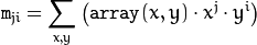
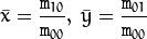
In case of a raster image, the spatial moments  are computed as:
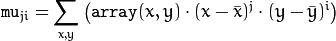
The central moments
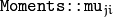 are computed as:
where
 is the mass center:
The normalized central moments
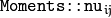 are computed as:
Note
 ,
,

 , hence the values are not stored.
The moments of a contour are defined in the same way but computed using the Green’s formula (see http://en.wikipedia.org/wiki/Green_theorem). So, due to a limited raster resolution, the moments computed for a contour are slightly different from the moments computed for the same rasterized contour.
See also
contourArea(), arcLength()
HuMoments
Calculates seven Hu invariants.
- C++: void HuMoments(const Moments& moments, double* hu)
- Python: cv2.HuMoments(m) → hu
- C: void cvGetHuMoments(const CvMoments* moments, CvHuMoments* hu)
- Python: cv.GetHuMoments(moments) → hu
Parameters: - moments – Input moments computed with moments() .
- hu – Output Hu invariants.
The function calculates seven Hu invariants (introduced in [Hu62]; see also http://en.wikipedia.org/wiki/Image_moment) defined as:
![\begin{array}{l} hu[0]= \eta _{20}+ \eta _{02} \\ hu[1]=( \eta _{20}- \eta _{02})^{2}+4 \eta _{11}^{2} \\ hu[2]=( \eta _{30}-3 \eta _{12})^{2}+ (3 \eta _{21}- \eta _{03})^{2} \\ hu[3]=( \eta _{30}+ \eta _{12})^{2}+ ( \eta _{21}+ \eta _{03})^{2} \\ hu[4]=( \eta _{30}-3 \eta _{12})( \eta _{30}+ \eta _{12})[( \eta _{30}+ \eta _{12})^{2}-3( \eta _{21}+ \eta _{03})^{2}]+(3 \eta _{21}- \eta _{03})( \eta _{21}+ \eta _{03})[3( \eta _{30}+ \eta _{12})^{2}-( \eta _{21}+ \eta _{03})^{2}] \\ hu[5]=( \eta _{20}- \eta _{02})[( \eta _{30}+ \eta _{12})^{2}- ( \eta _{21}+ \eta _{03})^{2}]+4 \eta _{11}( \eta _{30}+ \eta _{12})( \eta _{21}+ \eta _{03}) \\ hu[6]=(3 \eta _{21}- \eta _{03})( \eta _{21}+ \eta _{03})[3( \eta _{30}+ \eta _{12})^{2}-( \eta _{21}+ \eta _{03})^{2}]-( \eta _{30}-3 \eta _{12})( \eta _{21}+ \eta _{03})[3( \eta _{30}+ \eta _{12})^{2}-( \eta _{21}+ \eta _{03})^{2}] \\ \end{array}](../../../_images/math/16e925ec3fdbb385db38d28473ed74b82cde6b7b.png)
where
 stands for
 .
.
These values are proved to be invariants to the image scale, rotation, and reflection except the seventh one, whose sign is changed by reflection. This invariance is proved with the assumption of infinite image resolution. In case of raster images, the computed Hu invariants for the original and transformed images are a bit different.
See also
matchShapes()
findContours
Finds contours in a binary image.
- C++: void findContours(InputOutputArray image, OutputArrayOfArrays contours, OutputArray hierarchy, int mode, int method, Point offset=Point())
- C++: void findContours(InputOutputArray image, OutputArrayOfArrays contours, int mode, int method, Point offset=Point())
- C: int cvFindContours(CvArr* image, CvMemStorage* storage, CvSeq** firstContour, int headerSize=sizeof(CvContour), int mode=CV_RETR_LIST, int method=CV_CHAIN_APPROX_SIMPLE, CvPoint offset=cvPoint(0, 0) )
- Python: cv.FindContours(image, storage, mode=CV_RETR_LIST, method=CV_CHAIN_APPROX_SIMPLE, offset=(0, 0)) → cvseq
Parameters: - image – Source, an 8-bit single-channel image. Non-zero pixels are treated as 1’s. Zero pixels remain 0’s, so the image is treated as binary . You can use compare() , inRange() , threshold() , adaptiveThreshold() , Canny() , and others to create a binary image out of a grayscale or color one. The function modifies the image while extracting the contours.
- contours – Detected contours. Each contour is stored as a vector of points.
- hiararchy – Optional output vector containing information about the image topology. It has as many elements as the number of contours. For each contour contours[i] , the elements hierarchy[i][0] , hiearchy[i][1] , hiearchy[i][2] , and hiearchy[i][3] are set to 0-based indices in contours of the next and previous contours at the same hierarchical level: the first child contour and the parent contour, respectively. If for a contour i there are no next, previous, parent, or nested contours, the corresponding elements of hierarchy[i] will be negative.
- mode –
Contour retrieval mode.
- CV_RETR_EXTERNAL retrieves only the extreme outer contours. It sets hierarchy[i][2]=hierarchy[i][3]=-1 for all the contours.
- CV_RETR_LIST retrieves all of the contours without establishing any hierarchical relationships.
- CV_RETR_CCOMP retrieves all of the contours and organizes them into a two-level hierarchy. At the top level, there are external boundaries of the components. At the second level, there are boundaries of the holes. If there is another contour inside a hole of a connected component, it is still put at the top level.
- CV_RETR_TREE retrieves all of the contours and reconstructs a full hierarchy of nested contours. This full hierarchy is built and shown in the OpenCV contours.c demo.
- method –
Contour approximation method.
- CV_CHAIN_APPROX_NONE stores absolutely all the contour points. That is, any 2 subsequent points (x1,y1) and (x2,y2) of the contour will be either horizontal, vertical or diagonal neighbors, that is, max(abs(x1-x2),abs(y2-y1))==1.
- CV_CHAIN_APPROX_SIMPLE compresses horizontal, vertical, and diagonal segments and leaves only their end points. For example, an up-right rectangular contour is encoded with 4 points.
- CV_CHAIN_APPROX_TC89_L1,CV_CHAIN_APPROX_TC89_KCOS applies one of the flavors of the Teh-Chin chain approximation algorithm. See [TehChin89] for details.
- offset – Optional offset by which every contour point is shifted. This is useful if the contours are extracted from the image ROI and then they should be analyzed in the whole image context.
The function retrieves contours from the binary image using the algorithm [Suzuki85]. The contours are a useful tool for shape analysis and object detection and recognition. See squares.c in the OpenCV sample directory.
Note
Source image is modified by this function.
drawContours
Draws contours outlines or filled contours.
- C++: void drawContours(InputOutputArray image, InputArrayOfArrays contours, int contourIdx, const Scalar& color, int thickness=1, int lineType=8, InputArray hierarchy=noArray(), int maxLevel=INT_MAX, Point offset=Point() )
- Python: cv2.drawContours(image, contours, contourIdx, color[, thickness[, lineType[, hierarchy[, maxLevel[, offset]]]]]) → None
- C: void cvDrawContours(CvArr* img, CvSeq* contour, CvScalar externalColor, CvScalar holeColor, int maxLevel, int thickness=1, int lineType=8 )
- Python: cv.DrawContours(img, contour, externalColor, holeColor, maxLevel, thickness=1, lineType=8, offset=(0, 0)) → None
Parameters: - image – Destination image.
- contours – All the input contours. Each contour is stored as a point vector.
- contourIdx – Parameter indicating a contour to draw. If it is negative, all the contours are drawn.
- color – Color of the contours.
- thickness – Thickness of lines the contours are drawn with. If it is negative (for example, thickness=CV_FILLED ), the contour interiors are drawn.
- lineType – Line connectivity. See line() for details.
- hierarchy – Optional information about hierarchy. It is only needed if you want to draw only some of the contours (see maxLevel ).
- maxLevel – Maximal level for drawn contours. If it is 0, only the specified contour is drawn. If it is 1, the function draws the contour(s) and all the nested contours. If it is 2, the function draws the contours, all the nested contours, all the nested-to-nested contours, and so on. This parameter is only taken into account when there is hierarchy available.
- offset – Optional contour shift parameter. Shift all the drawn contours by the specified
 .
.
The function draws contour outlines in the image if
 or fills the area bounded by the contours if
 . The example below shows how to retrieve connected components from the binary image and label them:
#include "cv.h"
#include "highgui.h"

using namespace cv;

int main( int argc, char** argv )
{
    Mat src;
    // the first command-line parameter must be a filename of the binary
    // (black-n-white) image
    if( argc != 2 || !(src=imread(argv[1], 0)).data)
        return -1;

    Mat dst = Mat::zeros(src.rows, src.cols, CV_8UC3);

    src = src > 1;
    namedWindow( "Source", 1 );
    imshow( "Source", src );

    vector<vector<Point> > contours;
    vector<Vec4i> hierarchy;

    findContours( src, contours, hierarchy,
        CV_RETR_CCOMP, CV_CHAIN_APPROX_SIMPLE );

    // iterate through all the top-level contours,
    // draw each connected component with its own random color
    int idx = 0;
    for( ; idx >= 0; idx = hierarchy[idx][0] )
    {
        Scalar color( rand()&255, rand()&255, rand()&255 );
        drawContours( dst, contours, idx, color, CV_FILLED, 8, hierarchy );
    }

    namedWindow( "Components", 1 );
    imshow( "Components", dst );
    waitKey(0);
}
approxPolyDP
Approximates a polygonal curve(s) with the specified precision.
- C++: void approxPolyDP(InputArray curve, OutputArray approxCurve, double epsilon, bool closed)
- Python: cv2.approxPolyDP(curve, epsilon, closed[, approxCurve]) → approxCurve
- C: CvSeq* cvApproxPoly(const void* curve, int headerSize, CvMemStorage* storage, int method, double epsilon, int recursive=0 )
Parameters: - curve –
Input vector of a 2D point stored in:
- std::vector or Mat (C++ interface)
- Nx2 numpy array (Python interface)
- CvSeq or `` CvMat (C interface)
- approxCurve – Result of the approximation. The type should match the type of the input curve. In case of C interface the approximated curve is stored in the memory storage and pointer to it is returned.
- epsilon – Parameter specifying the approximation accuracy. This is the maximum distance between the original curve and its approximation.
- closed – If true, the approximated curve is closed (its first and last vertices are connected). Otherwise, it is not closed.
- headerSize – Header size of the approximated curve. Normally, sizeof(CvContour) is used.
- storage – Memory storage where the approximated curve is stored.
- method – Contour approximation algorithm. Only CV_POLY_APPROX_DP is supported.
- recursive – Recursion flag. If it is non-zero and curve is CvSeq*, the function cvApproxPoly approximates all the contours accessible from curve by h_next and v_next links.
- curve –
The functions approxPolyDP approximate a curve or a polygon with another curve/polygon with less vertices so that the distance between them is less or equal to the specified precision. It uses the Douglas-Peucker algorithm http://en.wikipedia.org/wiki/Ramer-Douglas-Peucker_algorithm
See http://code.ros.org/svn/opencv/trunk/opencv/samples/cpp/contours.cpp for the function usage model.
ApproxChains
Approximates Freeman chain(s) with a polygonal curve.
- C: CvSeq* cvApproxChains(CvSeq* chain, CvMemStorage* storage, int method=CV_CHAIN_APPROX_SIMPLE, double parameter=0, int minimalPerimeter=0, int recursive=0 )
- Python: cv.ApproxChains(chain, storage, method=CV_CHAIN_APPROX_SIMPLE, parameter=0, minimalPerimeter=0, recursive=0) → contours
Parameters: - chain – Pointer to the approximated Freeman chain that can refer to other chains.
- storage – Storage location for the resulting polylines.
- method – Approximation method (see the description of the function FindContours() ).
- parameter – Method parameter (not used now).
- minimalPerimeter – Approximates only those contours whose perimeters are not less than minimal_perimeter . Other chains are removed from the resulting structure.
- recursive – Recursion flag. If it is non-zero, the function approximates all chains that can be obtained from chain by using the h_next or v_next links. Otherwise, the single input chain is approximated.
This is a standalone contour approximation routine, not represented in the new interface. When FindContours() retrieves contours as Freeman chains, it calls the function to get approximated contours, represented as polygons.
arcLength
Calculates a contour perimeter or a curve length.
- C++: double arcLength(InputArray curve, bool closed)
- Python: cv2.arcLength(curve, closed) → retval
- C: double cvArcLength(const void* curve, CvSlice slice=CV_WHOLE_SEQ, int isClosed=-1 )
- Python: cv.ArcLength(curve, slice=CV_WHOLE_SEQ, isClosed=-1) → double
Parameters: - curve – Input vector of 2D points, stored in std::vector or Mat.
- closed – Flag indicating whether the curve is closed or not.
The function computes a curve length or a closed contour perimeter.
boundingRect
Calculates the up-right bounding rectangle of a point set.
- C++: Rect boundingRect(InputArray points)
- Python: cv2.boundingRect(points) → retval
- C: CvRect cvBoundingRect(CvArr* points, int update=0 )
- Python: cv.BoundingRect(points, update=0) → CvRect
Parameters: points – Input 2D point set, stored in std::vector or Mat.
The function calculates and returns the minimal up-right bounding rectangle for the specified point set.
contourArea
Calculates a contour area.
- C++: double contourArea(InputArray contour, bool oriented=false )
- Python: cv2.contourArea(contour[, oriented]) → retval
- C: double cvContourArea(const CvArr* contour, CvSlice slice=CV_WHOLE_SEQ )
- Python: cv.ContourArea(contour, slice=CV_WHOLE_SEQ) → double
Parameters: - contour – Input vector of 2D points (contour vertices), stored in std::vector or Mat.
- orientation – Oriented area flag. If it is true, the function returns a signed area value, depending on the contour orientation (clockwise or counter-clockwise). Using this feature you can determine orientation of a contour by taking the sign of an area. By default, the parameter is false, which means that the absolute value is returned.
The function computes a contour area. Similarly to moments() , the area is computed using the Green formula. Thus, the returned area and the number of non-zero pixels, if you draw the contour using drawContours() or fillPoly() , can be different.
Example:
vector<Point> contour;
contour.push_back(Point2f(0, 0));
contour.push_back(Point2f(10, 0));
contour.push_back(Point2f(10, 10));
contour.push_back(Point2f(5, 4));

double area0 = contourArea(contour);
vector<Point> approx;
approxPolyDP(contour, approx, 5, true);
double area1 = contourArea(approx);

cout << "area0 =" << area0 << endl <<
        "area1 =" << area1 << endl <<
        "approx poly vertices" << approx.size() << endl;
convexHull
Finds the convex hull of a point set.
- C++: void convexHull(InputArray points, OutputArray hull, bool clockwise=false, bool returnPoints=true )
- Python: cv2.convexHull(points[, hull[, returnPoints[, clockwise]]]) → hull
- C: CvSeq* cvConvexHull2(const CvArr* input, void* storage=NULL, int orientation=CV_CLOCKWISE, int returnPoints=0 )
- Python: cv.ConvexHull2(points, storage, orientation=CV_CLOCKWISE, returnPoints=0) → convexHull
Parameters: - points – Input 2D point set, stored in std::vector or Mat.
- hull – Output convex hull. It is either an integer vector of indices or vector of points. In the first case, the hull elements are 0-based indices of the convex hull points in the original array (since the set of convex hull points is a subset of the original point set). In the second case, hull elements aree the convex hull points themselves.
- storage – Output memory storage in the old API (cvConvexHull2 returns a sequence containing the convex hull points or their indices).
- clockwise – Orientation flag. If it is true, the output convex hull is oriented clockwise. Otherwise, it is oriented counter-clockwise. The usual screen coordinate system is assumed so that the origin is at the top-left corner, x axis is oriented to the right, and y axis is oriented downwards.
- orientation – Convex hull orientation parameter in the old API, CV_CLOCKWISE or CV_COUNTERCLOCKWISE.
- returnPoints – Operation flag. In case of a matrix, when the flag is true, the function returns convex hull points. Otherwise, it returns indices of the convex hull points. When the output array is std::vector, the flag is ignored, and the output depends on the type of the vector: std::vector<int> implies returnPoints=true, std::vector<Point> implies returnPoints=false.
The functions find the convex hull of a 2D point set using the Sklansky’s algorithm [Sklansky82] that has O(N logN) complexity in the current implementation. See the OpenCV sample convexhull.cpp that demonstrates the usage of different function variants.
ConvexityDefects
Finds the convexity defects of a contour.
- C: CvSeq* cvConvexityDefects(const CvArr* contour, const CvArr* convexhull, CvMemStorage* storage=NULL )
- Python: cv.ConvexityDefects(contour, convexhull, storage) → convexityDefects
Parameters: - contour – Input contour.
- convexhull – Convex hull obtained using ConvexHull2() that should contain pointers or indices to the contour points, not the hull points themselves (the returnPoints parameter in ConvexHull2() should be zero).
- storage – Container for the output sequence of convexity defects. If it is NULL, the contour or hull (in that order) storage is used.
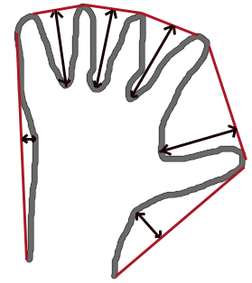
The function finds all convexity defects of the input contour and returns a sequence of the CvConvexityDefect structures, where CvConvexityDetect is defined as:
struct CvConvexityDefect
{
   CvPoint* start; // point of the contour where the defect begins
   CvPoint* end; // point of the contour where the defect ends
   CvPoint* depth_point; // the farthest from the convex hull point within the defect
   float depth; // distance between the farthest point and the convex hull
};
The figure below displays convexity defects of a hand contour:
fitEllipse
Fits an ellipse around a set of 2D points.
- C++: RotatedRect fitEllipse(InputArray points)
- Python: cv2.fitEllipse(points) → retval
- C: CvBox2D cvFitEllipse2(const CvArr* points)
- Python: cv.FitEllipse2(points) → Box2D
Parameters: points – Input 2D point set, stored in:
- std::vector<> or Mat (C++ interface)
- CvSeq* or CvMat* (C interface)
- Nx2 numpy array (Python interface)
The function calculates the ellipse that fits (in a least-squares sense) a set of 2D points best of all. It returns the rotated rectangle in which the ellipse is inscribed. The algorithm [Fitzgibbon95] is used.
fitLine
Fits a line to a 2D or 3D point set.
- C++: void fitLine(InputArray points, OutputArray line, int distType, double param, double reps, double aeps)
- Python: cv2.fitLine(points, distType, param, reps, aeps) → line
- C: void cvFitLine(const CvArr* points, int distType, double param, double reps, double aeps, float* line)
- Python: cv.FitLine(points, distType, param, reps, aeps) → line
Parameters: - points – Input vector of 2D or 3D points, stored in std::vector<> or Mat.
- line – Output line parameters. In case of 2D fitting, it should be a vector of 4 elements (like Vec4f) - (vx, vy, x0, y0), where (vx, vy) is a normalized vector collinear to the line and (x0, y0) is a point on the line. In case of 3D fitting, it should be a vector of 6 elements (like Vec6f) - (vx, vy, vz, x0, y0, z0), where (vx, vy, vz) is a normalized vector collinear to the line and (x0, y0, z0) is a point on the line.
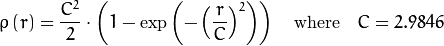
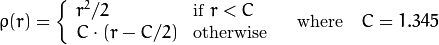
- distType – Distance used by the M-estimator (see the discussion below).
- param – Numerical parameter ( C ) for some types of distances. If it is 0, an optimal value is chosen.
- reps – Sufficient accuracy for the radius (distance between the coordinate origin and the line).
- aeps – Sufficient accuracy for the angle. 0.01 would be a good default value for reps and aeps.
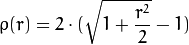
The function fitLine fits a line to a 2D or 3D point set by minimizing
 where
where
 is a distance between the
 point, the line and
 is a distance function, one of the following:
distType=CV_DIST_L2

distType=CV_DIST_L1

distType=CV_DIST_L12
distType=CV_DIST_FAIR

distType=CV_DIST_WELSCH
distType=CV_DIST_HUBER
The algorithm is based on the M-estimator (
http://en.wikipedia.org/wiki/M-estimator
) technique that iteratively fits the line using the weighted least-squares algorithm. After each iteration the weights
 are adjusted to be inversely proportional to
 .
.
isContourConvex
Tests a contour convexity.
- C++: bool isContourConvex(InputArray contour)
- Python: cv2.isContourConvex(contour) → retval
- C: int cvCheckContourConvexity(const CvArr* contour)
- Python: cv.CheckContourConvexity(contour) → int
Parameters: contour – Input vector of 2D points, stored in:
- std::vector<> or Mat (C++ interface)
- CvSeq* or CvMat* (C interface)
- Nx2 numpy array (Python interface)
The function tests whether the input contour is convex or not. The contour must be simple, that is, without self-intersections. Otherwise, the function output is undefined.
minAreaRect
Finds a rotated rectangle of the minimum area enclosing the input 2D point set.
- C++: RotatedRect minAreaRect(InputArray points)
- Python: cv2.minAreaRect(points) → retval
- C: CvBox2D cvMinAreaRect2(const CvArr* points, CvMemStorage* storage=NULL )
- Python: cv.MinAreaRect2(points, storage=None) → CvBox2D
Parameters: points – Input vector of 2D points, stored in:
- std::vector<> or Mat (C++ interface)
- CvSeq* or CvMat* (C interface)
- Nx2 numpy array (Python interface)
The function calculates and returns the minimum-area bounding rectangle (possibly rotated) for a specified point set. See the OpenCV sample minarea.cpp .
minEnclosingCircle
Finds a circle of the minimum area enclosing a 2D point set.
- C++: void minEnclosingCircle(InputArray points, Point2f& center, float& radius)
- Python: cv2.minEnclosingCircle(points, center, radius) → None
- C: int cvMinEnclosingCircle(const CvArr* points, CvPoint2D32f* center, float* radius)
- Python: cv.MinEnclosingCircle(points)-> (int, center, radius)
Parameters: - points –
Input vector of 2D points, stored in:
- std::vector<> or Mat (C++ interface)
- CvSeq* or CvMat* (C interface)
- Nx2 numpy array (Python interface)
- center – Output center of the circle.
- radius – Output radius of the circle.
- points –
The function finds the minimal enclosing circle of a 2D point set using an iterative algorithm. See the OpenCV sample minarea.cpp .
matchShapes
Compares two shapes.
- C++: double matchShapes(InputArray object1, InputArray object2, int method, double parameter=0 )
- Python: cv2.matchShapes(contour1, contour2, method, parameter) → retval
- C: double cvMatchShapes(const void* object1, const void* object2, int method, double parameter=0 )
- Python: cv.MatchShapes(object1, object2, method, parameter=0) → None
Parameters: - object1 – First contour or grayscale image.
- object2 – Second contour or grayscale image.
- method – Comparison method: CV_CONTOUR_MATCH_I1 , CV_CONTOURS_MATCH_I2 or CV_CONTOURS_MATCH_I3 (see the details below).
- parameter – Method-specific parameter (not supported now).
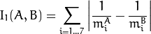
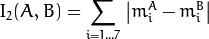
The function compares two shapes. All three implemented methods use the Hu invariants (see
HuMoments() ) as follows (
 denotes object1,:math:B denotes object2 ):
method=CV_CONTOUR_MATCH_I1
method=CV_CONTOUR_MATCH_I2
method=CV_CONTOUR_MATCH_I3
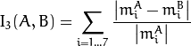
where
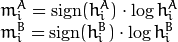
and
 are the Hu moments of
and
are the Hu moments of
and
 , respectively.
pointPolygonTest
Performs a point-in-contour test.
- C++: double pointPolygonTest(InputArray contour, Point2f pt, bool measureDist)
- Python: cv2.pointPolygonTest(contour, pt, measureDist) → retval
- C: double cvPointPolygonTest(const CvArr* contour, CvPoint2D32f pt, int measureDist)
- Python: cv.PointPolygonTest(contour, pt, measureDist) → double
Parameters: - contour – Input contour.
- pt – Point tested against the contour.
- measureDist – If true, the function estimates the signed distance from the point to the nearest contour edge. Otherwise, the function only checks if the point is inside a contour or not.
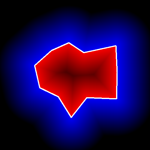
The function determines whether the point is inside a contour, outside, or lies on an edge (or coincides with a vertex). It returns positive (inside), negative (outside), or zero (on an edge) value, correspondingly. When measureDist=false , the return value is +1, -1, and 0, respectively. Otherwise, the return value is a signed distance between the point and the nearest contour edge.
See below a sample output of the function where each image pixel is tested against the contour.
| [Fitzgibbon95] | Andrew W. Fitzgibbon, R.B.Fisher. A Buyer’s Guide to Conic Fitting. Proc.5th British Machine Vision Conference, Birmingham, pp. 513-522, 1995. |
| [Hu62] |
|
| [Sklansky82] | Sklansky, J., Finding the Convex Hull of a Simple Polygon. PRL 1 $number, pp 79-83 (1982) |
| [Suzuki85] | Suzuki, S. and Abe, K., Topological Structural Analysis of Digitized Binary Images by Border Following. CVGIP 30 1, pp 32-46 (1985) |
| [TehChin89] | Teh, C.H. and Chin, R.T., On the Detection of Dominant Points on Digital Curve. PAMI 11 8, pp 859-872 (1989) |
Help and Feedback
You did not find what you were looking for?- Ask a question in the user group/mailing list.
- If you think something is missing or wrong in the documentation, please file a bug report.